


ABC inventory classification has been around so long that most planners just assume it’s the only way to segment inventory. In fact, it’s not. And it’s not even nearly the best way. It’s actually a throwback from technology developed during the 1960s that hasn’t responded to the orders of magnitude increase in computer power that has enabled far better ways of solving the problem.
In this blogpost we will look into a more detailed explanation of why ABC inventory classification is old school and look at what true inventory optimization in 2021 looks like.
Understanding the basics of ABC inventory classification
To understand the shortcomings of ABC inventory classification, we need to understand how it is done. Nearly all traditional inventory management applications calculate safety stock for each individual SKU-Location combination. This requires identifying the desired service level % for each SKU-Location.
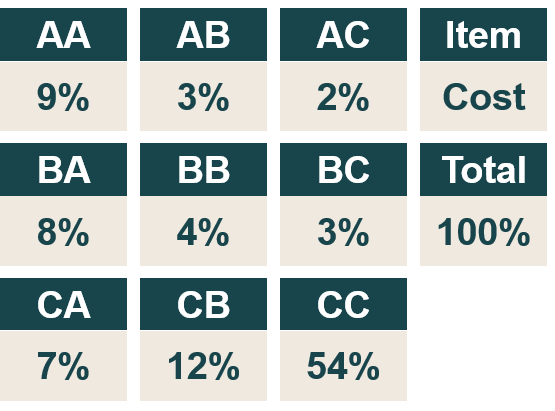
Since most companies have tens of thousands, hundreds of thousands, or even millions of combinations, it’s impossible to identify a service level for every individual SKU-Location. So a simplification is necessary and ABC classification is one way of doing it. A common method is a 3×3 matrix with the cost value on the Y axis and order-lines on the X axis, a so called “double” ABC classification.
The percent distribution between classes is often based on 80% of the cost value in the A items, 15% in the B items and 5% in the C items. The same 80/15/5 breakdown is applied to the number of order-lines. Because just a few items can generate so many order-lines and cost of sales, it usually only takes a few A items to reach the 80% thresholds. Therefore, the end result is a matrix with a very small share classified as AA and a majority classified as CC.
A ”trial & error” process is then used to allocate a desired service level to each ABC class. The AA class is often given the highest service level and the CC class the lowest. The aggregated service level is calculated and might end up at 94% in the first try, which might not fit the company’s overall goal, such as 95%. To reach the 95% goal, iterative attempts are made using higher service levels for one or several classes (and perhaps reducing some). The new distribution might turn into an aggregated service level of 95.5%. A small buffer (0.5% in this case) is often good, and the service levels for each class are confirmed.
From here, all of the items (or articles) in each ABC class are assigned the same service level target. If we have 10,000 items in stock, then 5400 in the CC class will be assigned the same service level target. Then the safety stock levels are calculated which results in a total inventory investment.
The pitfalls of ABC Inventory classification
Let us think about this for a moment. Inventory investment is a consequence of each ABC classes’ service level. Could we have chosen other service levels for the classes and still reach 95.5%? Of course! There are a large number of combinations that could result yield the same result.
How do we then know that the distribution we chose is the most optimal one, achieving a minimum stock investment? The answer is that we don’t know. That is why this method is called ”inventory management” rather than ”inventory optimization”.
Supply Chains are complex, with several connected echelons such as central, regional and local inventories. Also some traditional inventory management software offer an 8×8 ABC matrix per location. The workload to define and continuously maintain these matrices becomes very intense. And, as we said, we don’t know whether or not we have an optimal distribution.
What “best in class” inventory Segmentation looks like today
Is there another way to address safety stock computing in 2021? The answer is, of course, yes. A more modern approach exists.
Traditional ABC classification is based on an operational or logistics perspective. There is rarely any connection to sales and marketing or the companies’ customer needs.
Inventory optimization instead looks at the product range and the business. This difference is possible thanks to the use of “service class”. Examples of service classes can be ”accessories”, ”items with a high margin”, ”own-brands”, ”high end brands”, ”critical spare parts”, to name a few. This type of categorization is much more relevant to sales and marketing, who often have very little or no understanding of ABC classification. Every service classification contains items from several ABC classifications (according to the old method) which is irrelevant to true inventory optimization.
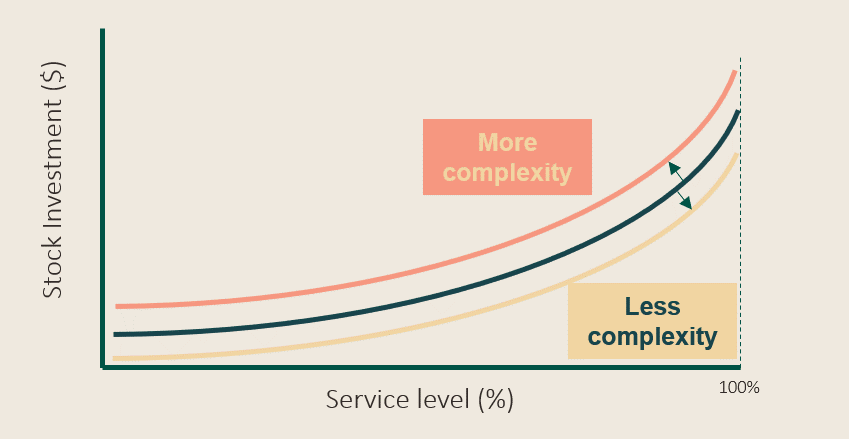
Just as in traditional inventory management, aggregated service level goals are also defined in inventory optimization, but per service class instead of ABC class. What happens in the following steps is very different from traditional inventory management. By using ”stock-to-service” curves, the software optimizes every single service level and safety stock level of the SKU-Location, which is also known as mix optimization.
The aggregated service class goal is achieved with a stock investment as low as possible. Instead of inventory planning with ABC classes, every SKU-Location gets a service level to calculate safety stock levels. The inventory optimization software automatically calculates a service level for every SKU-Location that aggregates to the total service level target for the overall service class, achieving “service level optimization“.
True inventory optimization uses “stock-to-service”
True inventory optimization models every SKU-Location and summarizes it in a ”stock-to-service” efficient frontier, where the relationship between service level and stock investment are defined. If demand variation or lead time increases, the stock investment (or complexity) must be increased in order to keep the same service level and vice versa.
The result is that every single item in every single location (SKU-Location) is an individual and is analysed and managed as such. In a sense, there can be as many ABC classifications as there are SKU-Location combinations.
This statement is impossible to fit into traditional inventory management and so it is a very challenging one to accept. If every SKU-Location combination was described with dozens of variables (demand variation, standard cost, my order quantity, multiple order quantity, run-out time, lead time, variation in lead time, sustainability, and more), it would unmanageable, instead of just one or two dimensions, as in a traditional ABC classification matrix.
By the way, it’s important to point out that the automated differentiation of service levels in each service class can be set within defined limits. As an example, the aggregated service level goal for “accessories” could be 93% with a lower limit of 89%. The inventory optimization can then subscribe any service level from 89% and above in a way that the stock investment is minimized. For example, “critical spare parts” could have a goal of 99.5% with a lower limit of 99.3%. Reducing the degrees of freedom in each service class (or increasing number of service classes) will lessen the potential of inventory reduction, since competition is reduced. But these reductions in freedom are not critical as long as they aligns with company strategies and customer demands.
Truly modern inventory optimization enables a whole new level of automation of large complex supply chains with hundreds of thousands of SKU-Location combinations where service levels can be guaranteed over time with a minimum of stock investment.